Recommended Reading from the Fed

There are two particularly good reads posted by Federal Reserve economists today. The first is "Deleveraging: Is it over and what was it?" by Claudia Sahm. The role of household deleveraging in the Great Recession has been heavily emphasized, notably at Atif Mian and Amir Sufi's very good new "House of Debt" blog. Sahm summarizes three new research papers on the topic of household deleveraging. The papers address three big questions:

1. When will deleveraging be over?
2. What do households do when they can't repay their debts?
3. Whose decision is deleveraging anyway?

The research on Question 2 is especially interesting:

"Given the increase in mortgage defaults in this recession, it took unusually long (averaging up to 3 years in some states) to go from initial delinquency to a completed foreclosure on a home. During the foreclosure process, households typically lived 'rent free' in their homes. So what did these households do with the extra cash? The authors find a significant improvement in the performance of credit card debt (reduced delinquency and lower balances). Although these households were under considerable financial stress and were already facing a huge hit to their credit scores due to a foreclosure, they used some of the freed up money to pay off their other debts...Normally economists think that if you give cash to households who are financially constrained they will spend it not use it to service debt."

Sahm's overall takeaway from the research she reviews is that:

"There was a big hit to 'permanent income' (households' expected lifetime income and net worth) and credit availability. Thus the level of spending and debt that made sense for households changed dramatically with the recession. Economists already understood this adjustment in the standard consumption framework even if the size and persistence of the shocks have been surprising. So in this sense "deleveraging" is simply a new way to frame the issue rather than a new behavior. And yet, we saw that the debt obligations that households made when everyone thought they were richer could not be easily undone."

Another Fed post worth reading today is a speech, "A Review of the Experience of Fielding the Survey of Consumer Expectations," by James McAndrews. The New York Fed's Survey of Consumer Expectations (SCE) is a relatively new monthly survey of consumers' inflation, labor market, and household finance expectations.

The effort that the NY Fed has devoted to developing this survey is testament to the increasing emphasis economists are placing on understanding the links between expectations and the economy. (This is near and dear to me, as a theme of my dissertation.) Expectations have long played a role in macroeconomic models, but are sometimes treated as an afterthought, probably because they can be difficult to observe and quantify. The SCE includes probabilistic survey questions, which ask respondents to describe their probability distribution over future outcomes. This reveals the uncertainty associated with consumers' expectations.

In the speech, McAndrews delves into some of the nitty-gritty of the multi-year survey development process, which is quite fascinating. He also summarizes the past research using the survey data.

Cab Drivers, Preachers, and Economists' Wives

Lately I have been working on a Great Depression-era economic history paper to constitute one chapter of my dissertation. The practice of writing a history paper is highly enjoyable. It can send you deep into the (thankfully in my case mostly digital) archives. For younger scholars, it is one of the best ways to learn about and reflect on your chosen profession. This can sometimes be quite humorous.

Irving Fisher was a Yale professor and one of the best-known economists of the early 20th century. His weekly Business Page, the closest thing to an economics blog of the time, was widely syndicated in newspapers across the country. His modern day counterpart greatly praises his debt deflation theory, and deservedly so. In addition to good insights, Fisher had many good lines.

The best came at a meeting of the American Academy of Political and Social Sciences in November 1933. Picture Fisher at the podium about to make the closing remarks for the meeting. He begins,

"It is more than fair of the presiding officer to give me not only the first word, but the last word."

(One of the other speakers was a United States Senator, by the way.) Maybe it doesn't take an economist to think this way, but it takes one to speak this way. This is just some relatively benign self-aggrandizement, and a good ego is always good for a good laugh. Another quote, from the 1971 Journal of Money, Credit, and Banking, also made me laugh, but seemed less benign.

"Who among us [economists] has not listened politely to the bizarre theories of the Great Depression as proffered by cab drivers, preachers, and (worst of all) economists' wives? One simply learns to avoid cabs, churches, and home each time the Grapes of Wrath makes one of the film festivals or books by Studs Terkel about Huey P. Long make the best-seller lists."

Fisher only asserts his superiority to other economists and politicians, whereas this economist asserts economists' intellectual superiority to the public at large, or at least its female and service professional components. "Isn't it cute when our wives try to understand the economy? Aren't we great for being so polite to the poor dolts?"

Now, the vast majority of economists I know today have the utmost respect for their spouses' intellects. What we should avoid at all costs is a "polite" disregard of the intellect of the general public. Economists shouldn't "avoid cabs, churches, and home." Cabs, churches and home are the economy. (And I can think of one particular preacher whose vision of economics will not be ignored.) Economic policy would function more smoothly if more people understood it. In a democracy, people deserve the chance to understand the economy and economic policies that affect their lives. This is put really well by Alan Blinder and coauthors (2009), regarding monetary policy:

"It may be time to pay some attention to communication with the general public...In the end, it is the general public that gives central banks their democratic legitimacy, and hence their independence."

This is also why I really respect efforts like those of Annamaria Lusardi to teach economic and financial literacy to the public under the assumption that everyone is capable of understanding, so long as they are given the opportunity to learn.

Long-Term Unemployment and the Dual Mandate

The Federal Reserve's mandate from Congress, as described in the Federal Reserve Act, is to promote "maximum employment, stable prices, and moderate long-term interest rates." In January 2012, the FOMC clarified that a PCE inflation rate of 2% was most consistent with the price stability part of the so-called "dual mandate." The FOMC's Statement on Longer-Run Goals and Monetary Policy Strategy says:

In setting monetary policy, the Committee seeks to mitigate deviations of inflation from its longer-run goal and deviations of employment from the Committee's assessments of its maximum level. These objectives are generally complementary. However, under circumstances in which the Committee judges that the objectives are not complementary, it follows a balanced approach in promoting them, taking into account the magnitude of the deviations and the potentially different time horizons over which employment and inflation are projected to return to levels judged consistent with its mandate.

Lately, PCE inflation has been well below 2%. There is no similarly-specific definition of maximum employment, but I think it is safe to say that we are not there yet. So we seem to be in a situation in which the objectives are complementary--employment-boosting policies that also put some upward pressure on prices would get us closer to maximum employment and stable prices at the same time. This is supposed to be the "easy case" for monetary policymakers, earning the name "divine coincidence." The tougher case would come if inflation were to get up to or above 2% and employment were still too low. Then there would be a tradeoff between the employment and price stability objectives, making the Committee's balancing act more difficult.

San Francisco Federal President John Williams presents the case that the rise in the share of long-term unemployment should affect the approach that Committee members take when faced with such a balancing act. Williams and SF Fed Economist Glenn Rudebusch have a new working paper called "A Wedge in the Dual Mandate: Monetary Policy and Long-Term Unemployment." In this paper, they document key empirical facts about the share of long-term unemployment and explain how it alters the relationship between employment and inflation.

Source: Rudebusch and Williams 2014, p. 4.

First, the key empirical facts about long-term unemployment share in the U.S.:

1. It has trended upward over the past few decades.
2. It is countercyclical.
3. Its countercyclicality has increased in recent decades.

Fact 1 has been attributed to the aging population, women's rising labor force attachment, and increasing share of job losses that are permanent separations rather than temporary layoffs (Groshen and Potter 2003, Aaronson et al. 2010, Valletta 2011).

The long-term unemployed appear to place less downward pressure on wages and prices than the short-term unemployed. This may be because the long-term unemployed are less tied to the labor market and search less intensely for a job as they grow discouraged (e.g., Krueger and Mueller 2011). Stock (2011) and Gordon (2013) find that distinguishing between long- and short-term unemployment can help account for the puzzling lack of disinflation following the Great Recession. Rudebusch and Williams find a similar result by running Phillips Curve regressions that include short-term and long-term unemployment gaps as regressors. Only the coefficient on the short-term unemployment gap is negative and statistically significant, implying that short-run unemployment exerts downward pressure on prices while long-run unemployment does not.

The finding that long-term and short-term unemployment have different implications for price dynamics is very relevant for the Fed's pursuit of its dual mandate.  When the long-term unemployment share is high, this introduces a "wedge" between the employment and price stability portions of the mandate. Employment and inflation won't be as prone to moving in the same direction, because employment can get very low without much downward pressure on wages (and prices). To formalize what this means for monetary policy decisions, Rudebusch and Williams build a stylized model economy (skip ahead if not interested in the details) in which the central bank's objective is to minimize a quadratic loss function:
\begin{equation}
L=\tilde \pi + \lambda \tilde u,
\end{equation}
where pi tilde and u tilde are deviations of inflation from its target and unemployment from the natural rate, and lambda is the weight that policymakers place on unemployment stabilization versus inflation stabilization. Let the unemployment deviation depend on a demand shock v and the deviation of the short-term interest rate from the natural rate (IS equation):
\begin{equation}
\tilde u = \eta \tilde i + v
\end{equation}
 Let deviations in inflation depend on an inflation shock e and the deviation of the short-run unemployment rate s from its natural rate:
\begin{equation}
\tilde \pi = -\kappa \tilde s + e
\end{equation}
The short-run unemployment rate is a fraction of the overall unemployment rate u,
\begin{equation}
s=\theta u,
\end{equation} where
\begin{equation}
\theta=\bar \theta -\delta \tilde u + z,
\end{equation}
where z is a shock to the short-run unemployment share. If we substitute these equations into the loss function and take first order conditions, we arrive at an expression for the optimal deviation of inflation from its target:
\begin{equation}
\tilde \pi*=\frac{\lambda}{\lambda+\kappa^2 \theta^2}e-\frac{\lambda \kappa \bar u}{\lambda+\kappa^2 \theta^2}z
\end{equation}

The first thing to notice here is that the demand shock v does not show up in the optimal policy decision. This is the divine coincidence-- demand shocks impose no tradeoff between the employment and inflation objectives.

The second thing to notice is how the inflation shock e and the short-run unemployment share z. The first term is standard, and shows how the optimal policy partially offsets a positive (negative) inflation shock by raising (lowering) unemployment. The other term is new to this paper. A positive shock to theta acts like a negative inflation shock in the sense of prescribing a higher short-run unemployment rate and lower inflation rate. Another policy implication arises because theta affects the slope of the Phillips curve with respect to aggregate unemployment. This creates an asymmetry in the optimal policy response to inflation shocks that depends on theta.

During the Great Recession, the short-run unemployment share theta reached historic lows. Rudebusch and Williams simulate their model starting in the first quarter of 2014, using actual data from 2013 as initial conditions. They compare the optimal policy response implied by their model to that implied by a standard model (i.e. one that does not distinguish between short-run and long-run unemployment). The figure below displays the results. The quantitative results are not meant to be taken too seriously, since the models involve drastic oversimplifications, but the qualitative differences are  illustrative.The model that distinguishes between short-run and long-run unemployment (shown as black lines) prescribes a higher inflation rate--temporarily above 2%--than the standard model (shown as dashed red lines).

Source: Rudebusch and Williams 2014, p. 22

The authors conclude (emphasis added):

During the recent recession and recovery, the number of discouraged jobless excluded from the unemployment rate and the number of part-time employees wanting full-time work have reached historic highs. If the true measure of labor underutilization included these individuals, even though they have little or no eff ect on wage and price setting, then the wedge in the Fed's dual mandate would be even wider. Based on the analysis in this paper, the implications are clear: Optimal policy should trade off a transitory period of excessive inflation (beyond what is calculated using this paper's model) in order to bring the broader measure of underemployment to normal levels more quickly.

This is a very interesting and intuitive result, and is highly relevant to the policymaking environment in both the United States and elsewhere, particularly Europe. However, I'm not sure that the FOMC as a whole will take this paper's implications seriously. The committee does not share a single "loss function" like the quadratic function presented in the paper, which treats overshooting and undershooting of the inflation target symmetrically. Mark Thoma's comment on the paper is, "I'll believe the Fed will allow *intentional overshooting* of its inflation target when I see it."

Kocherlakota's Case for Price Level Targeting

Narayana Kocherlakota, President of the Federal Reserve Bank of Minneapolis, described the benefits of price level targeting to the Economic Club of Minnesota on May 21. He began by explaining that Congress has charged the FOMC with making monetary policy to promote price stability and maximum employment. Since January 2012, the FOMC has interpreted an inflation rate of 2% as most consistent with the price stability part of the mandate.

Since the adoption of the 2% inflation target, inflation, as measured by the annual change in the price index for personal consumption expenditures, has actually been just above 1%. Kocherlakota agrees with the Congressional Budget Office forecast that inflation will not reach 2% until around 2018. He explains why below-target inflation is a problem:

"The low inflation in the United States tells us that resources are being wasted. What exactly are these wasted resources? ...the biggest and most disturbing answer is our fellow Americans. There are many productive people in the United States available to work more hours, and our society is deprived of their production. 

This key point is generally underappreciated. I’ve said that the FOMC is undershooting its price stability objective and is expected to continue to do so. But we should all keep in mind that this outcome—and especially the forecast for continued undershooting—typically means that the FOMC is also underperforming on its other objective of promoting maximum employment."

Kocherlakota notes that "the downside misses with respect to inflation cumulate into a significantly lower price level. If my inflation forecast is right, the price level in 2018 will be about 2.5 percent below what it would have been had the FOMC hit its inflation target over the preceding six years." Then he asks, "How should the FOMC’s inflation goals in the years following 2018 be influenced by the undershooting of the inflation target in the preceding years?"

He describes two main benefits of adopting price level targeting, instead of inflation targeting. (His disclaimer: "I won’t take a stand today on which of those approaches is better. My goal is simply to initiate a policy conversation about future—indeed, possibly far-off future—monetary policy choices.") With price level targeting, the central bank targets a set path for the price level, rather than a set rate of change in the price level. If an inflation-targeting central bank undershoots its 2% target one year, it will still target 2% the next year. A price level-targeting central bank could target a path for the price level with a 2% growth rate, but if inflation is less than 2% one year, it will need to be above 2% the next year to get the price level back up to the targeted path. Here are Kocherlakota's two reasons why price level targeting could be a better option:

"The first reason is that price level targeting makes long-term contracts safer for borrowers and lenders. For example, suppose a family took out a 30-year mortgage in 2012, under the expectation that the FOMC would deliver on its commitment to keep inflation at 2 percent. Because inflation has been so low over the past two years, the borrower’s current repayments are now surprisingly expensive in real terms...The FOMC can’t solve that problem today, But if the FOMC uses inflation targeting, the borrower’s repayments are likely to remain surprisingly expensive in real terms even in 2042...In contrast, if the FOMC uses price level targeting, the borrower’s repayments in 2042 are likely to be close, in real terms, to what the borrower expected when originally taking on the loan. 

The second reason that the FOMC might want to use price level targeting is that it would serve as an automatic stabilizer for the economy. As I described earlier, when demand is low, inflation tends to be below target. With price level targeting, the FOMC makes up for low inflation by using monetary policy to stimulate higher future inflation and higher future demand. But this prospect of higher future demand is an incentive for businesses to hire and invest more now. Thus, with price level targeting, the FOMC’s anticipated future policy choices automatically offset current adverse shocks."

I don't think a switch to price level targeting is likely in the near term. It would (nearly) be a global first. Only the Swedish Riksbank, from 1931-37, has explicitly targeted the price level. The Bank of Canada, an inflation-targeting regime since 1991, seriously considered switching to price level targeting, but decided against it in 2011.

Meanwhile, other Fed officials and researchers claim that in practice, the FOMC has behaved as if it were price level targeting. St. Louis Fed President James Bullard notes that if we take the 1995 price level and project a 2 percent inflation price level path from that point forward, the actual U.S. price level close to this path. Similarly, Dave Altig and Mike Bryan at the Atlanta Fed calculate that "If you accept that the Fed, for all practical purposes, adopted a 2 percent inflation objective sometime in the early to mid-1990s, there arguably really isn't much material distinction between its inflation-targeting practices and what would have likely happened under a regime that targeted price-level growth at 2 percent per annum. The actual price level today differs by only about 0.5 to 1.5 percentage points from what would be implied by such a price-level target." They explain:

"In principle, there is no reason why a central bank consistently pursuing an inflation target can't deliver the same outcomes as one that specifically and explicitly operates with a price-level target. Misses with respect to targeted inflation need not be biased in one direction or another if the central bank is truly delivering on an average inflation rate consistent with its stated objective."

In other words, they are saying that since inflation targeting allows base drift and price level targeting does not, but as long as base drift averages out to zero, there is not much difference. Since the early to mid-90s, the FOMC has approximately balanced out its overshooting and its undershooting of 2% inflation. This is an average over several business cycles, though, so the automatic stabilizer benefits that Kocherlakota mentions would not have been reaped. This also includes the years before the Fed adopted its explicit 2% inflation target. It seems like there was greater willingness to let inflation go above 2% when the target was not explicit. Mark Thoma has noted that comments made by some Fed officials could indicate that the Fed viewed the costs of overshooting and undershooting its target as asymmetric--that the target is actually more of a ceiling. If this is the case, than misses with respect to targeted inflation will likely be biased downward. A shift to treating the target as a true target, with symmetric costs of overshooting and undershooting, and sufficient weight on the employment part of the mandate, may be an easier-to-implement solution than an explicit price-level target.

A Reply to "Does Inflation Make You Poorer?"

Noah Smith channels Robert Shiller circa 1997 in his recent post, "Does Inflation Make you Poorer?" While Noah asks this question rhetorically, Shiller actually asked a series of related questions in a questionnaire of 677 people. His sample included both economists and non-economists from the U.S., Brazil, and Germany. He found:

"Among non-economists in all countries, the largest concern with inflation appears to be that it lowers people’s standard of living. Non-economists appear often to believe in a sort of sticky-wage model, by which wages do not respond to inflationary shocks, shocks which are themselves perceived as caused by certain people or institutions acting badly. This standard of living effect is not the only perceived cost of inflation among non-economists: other perceived costs are tied up with issues of exploitation, political instability, loss of morale, and damage to national prestige."

The first concern is the subject of Noah's mockery. True, some people think in partial equilibrium, neglecting the effects that inflation might have on their nominal income. But it is not an unreasonable concern in some contexts. Nominal wage stagnancy is a reality for many workers. In a 2008 Pew Survey, 57% of respondents believed that their income was rising slower than the cost of living.

In the figure below, the CPI, average hourly earnings for all private sector workers, and average hourly earnings for retail trade employees are all plotted. All are normalized to 100 in 2006. While average hourly earnings for all workers have grown faster than the CPI, the opposite is true for workers in retail. Since 2006, the price level is about 21% higher, but hourly wages in retail are less than 11% higher. They feel poorer and they are poorer.

Did inflation "make them poorer?" Not directly. But the political economy of inflation certainly contributed. Prices and wages do not simply rise or fall on their own. People choose to raise or lower them--this is why prices and wages are in the domain of economics, after all. Who chooses, and how do they choose? That's where things get more complicated. Decision-makers at firms set prices subject to an almost innumerable set of constraints and considerations imposed by the institutional and policy environment they face. Wages are not simply set by some abstract market-clearing condition; they involve bargaining between firms and individual employees or labor unions. Regulations, policy, and social norms also affect the bargaining powers of the relevant groups, with palpable effects on the wage structure.

Source: http://research.stlouisfed.org/fred2/graph/?g=y1d

In Japan, for example, deflation has plagued the economy for years. When Shinzo Abe ushered in a return to positive inflation, most Japanese consumers described rising prices as "rather unfavorable." These consumers were not being unreasonable. They were getting poorer! When prices started rising, wages did not. Since the 1950s, Japanese salaries have been determined by coordinated negotiations between unions and large employers. Only very recently, with the backing of Abe, have the unions had sufficient bargaining power to raise salaries in these negotiations. Japan also has a growing informal sector, where already-low nominal wages are unlikely to rise with the price level. Maybe eventually the overall Japanese economy will grow so much that even the low-wage informal workers will be better off. But no one knows how long that could take. Noah says it himself: "Whenever you buy something, the money you spend is someone else's income." But we don't know whose income it will be.

This is not to say that Japanese deflation was a good thing or made people richer. Quite the opposite. But it is to say that people should complain when their cost of living is rising faster than their earnings. Inflation has distributional effects, which will tend to benefit the politically powerful. The people getting the short end of the deal are perfectly rational to be upset about it, especially if their dissatisfaction can be harnessed into political action.

Not only inflation itself, but also inflation risk, has costs and distributional effects. The unpredictability of inflation is part of its cost. Hedging against inflation is theoretically possible but difficult. Inflation risk is costly for its bearers. Our political and economic institutions determine who the bearers will be. When social security and pensions are indexed to the price level, inflation risk to pensioners is reduced, while inflation risk to pension funds increases. When private debt contracts are primarily nominal, an unexpected increase in inflation will be costly for creditors. Indexing sovereign debt to the price level also redistributes inflation risk between countries and their creditors.

The other perceived costs of inflation that Shiller lists--exploitation, political instability, loss of morale, and damage to national prestige--all have historical precedents and are also related to the political economy of inflation. A government that "inflates away its debts" risks imposing any or all of these costs.  These costs of inflation are less relevant in the low inflation environments of the United States and much of Europe today. An increase in inflation from, say, 1% to 3% is unlikely to foster political instability or erode national prestige.

In the U.S. today, I think a little more inflation would be a good thing. But I think we also should take seriously the concerns of people whose real income is falling for one reason or another. This boils down to another call for economists to keep worrying about inequality-- even when thinking about issues like inflation.

Guest Post by John Mondragon: Keeping Up with the Joneses and Household Debt

This guest post was contributed by John Mondragon, an economics PhD candidate at Berkeley. He is the coauthor of a working paper that is closely related to my recent post on consumption contagion and income inequality. I'm very excited that he has agreed to contribute this post about the working paper. John is on Twitter @Mondragon_John. 

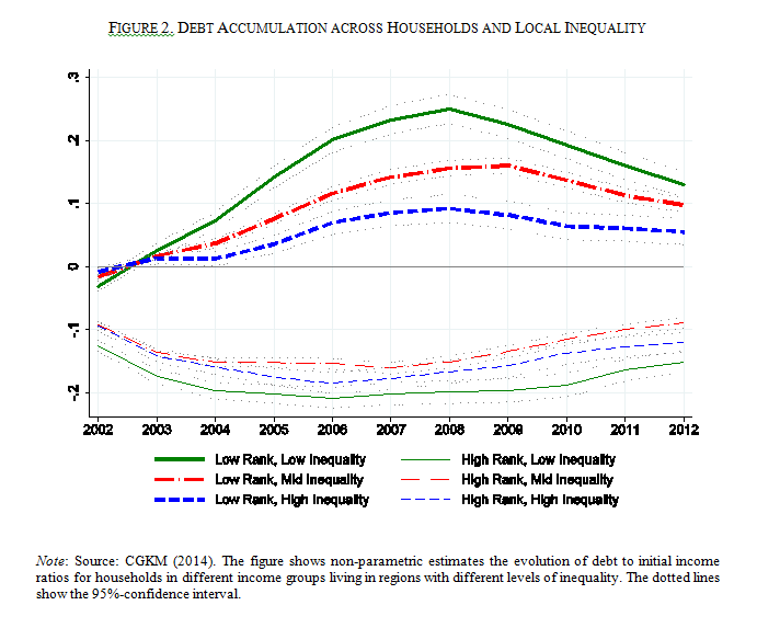
Since the 1980s U.S. households have dramatically increased the amount of debt they hold. One frequent explanation for this trend is that the large increase in income inequality over this same period caused households to borrow more (see Figure 1). The intuition is that low-income households attempted to “keep up” with the increasing consumption of their high-income neighbors. This could affect debt levels if the low-income household decides to fund its consumption by leveraging with debt (as opposed to increasing labor supply or drawing down assets). This type of behavior is often referred to as “keeping up with the Joneses”, consumption cascades, consumption spillovers, or external habit.

In a working paper I have with Olivier Coibion, Yuriy Gorodnichenko, and Marianna Kudlyak we look at whether, in the years running up to the financial crisis as well as during the Great Recession, low-, middle-, and high-income households accumulated different amounts of debt (relative to their incomes)  depending on the level of income inequality in their region. Our main finding is that low-income households in high-inequality areas increased their leverage by less than similar households in low-inequality areas. Our non-parametric results in Figure 2 suggest that a household in the bottom third of the income distribution within their area and inequality distribution across areas increased their leverage by around 15 percentage points more than a similar household in the top third of the inequality distribution in the years immediately prior to the financial crisis. This is the exact opposite effect one would expect if “keeping up with the Joneses” was the primary cause of borrowing by low-income households.

Because our data (see Additional Details below) allow us to break debt into pieces, we can examine which types of debt are driving these differences. While we find similar patterns for mortgage debt, auto debt, and credit card limits as those documented for total debt accumulation, we find no systematic differences across households and inequality regions in terms of their credit card balances. Since credit card limits primarily reflect credit supply conditions whereas credit card balances reflect households’ demand for credit, we interpret the difference in results across credit card limits and balances as pointing toward credit supply factors as the root cause of the link between inequality and borrowing.

The intuition is simple. First, lenders confront asymmetric information as they try to infer which borrowers are less likely to default. Second, high-income borrowers are less likely to default so lenders use income as a way to infer borrower type. In a perfectly equal income distribution all borrowers are equally likely to be a high or low default risk. But as inequality increases and the income difference between low- and high-income borrowers becomes larger, high-risk and low-risk borrowers are easier to tell apart when they reveal their incomes to banks. Lenders will then be able to offer cheaper and more readily accessible credit to high-income/low-risk borrowers as well as more likely to deny loans to low-income/high-risk borrowers. To test these predictions we use data from the Home Mortgage Disclosure Act (HMDA) which requires mortgage lenders to report details on applications including whether a loan was denied, the size of the loan, income of the applicant, and other characteristics. We find that low-income applicants are more likely to be denied mortgages and to be charged a high interest rate in high-inequality areas relative to similar applicants in low-inequality areas. Thus, this evidence also supports a credit supply interpretation of the link between local income inequality and differential borrowing patterns across income groups that is at odds with the “keeping up with the Joneses” interpretation.

Part of the reason I was invited to write here was to discuss the differences between our results and those in a recent paper by Bertrand and Morse, because their empirical findings do provide evidence of “keeping up with the Joneses” forces. There are at least two important differences. First, their outcome is consumption while ours is debt. It is possible that low-income households funded their consumption with changes in labor supply, savings, or even some debt. But our results tell us that any use of debt in this way cannot be the primary story of inequality and debt accumulation during this period. This is important to note because debt accumulation was central to the creation of many of the financial assets behind the financial crisis. Second, Bertrand and Morse use changes in consumption among the wealthy as their explanatory variable while we use inequality. It is possible that in some areas the consumption differences between households are not as large as in other areas even though both have the same measured inequality. This can occur if there is variation in precautionary savings, the “visibility” of consumption bundles, or the proximity of high- and low-income households. As the relationship between high-income household consumption and measured inequality becomes more complex our results become less directly comparable.

Thanks very much to Carola for having us!

Additional Details

The data we use for our primary results are from the New York Federal Reserve Bank Consumer Credit Panel/Equifax (referred to as the CCP), which provides comprehensive debt measures for millions of U.S. households since 1999. Because these data do not include income we impute incomes using the relationship between common observables in the Survey of Consumer Finances. Using these imputed incomes we construct measures of local inequality, household positions in the income distribution, and household debt-to-income ratios. We are able to check our measures of inequality and rank against various external measures and find they are very highly correlated.

Our results are robust to the level at which we measure inequality (zip, county, state), the measure of inequality we use (ratio of log incomes at the 90th and 10th percentile from the CCP, Gini coefficients from the IRS and Census data), an extensive set of household and area controls, and numerous splits of our sample. In particular our results hold within subsamples defined according to house price appreciation, average credit scores, income levels, initial debt ratios, and geographic regions.

Consumption Contagion and Income Inequality

The trends of rising income inequality and the declining national savings rate since the early 1980s may be related, according to a paper by Marianne Bertrand and Adair Morse. The authors find that higher levels of visible consumption by increasingly better-off households at the top of the income distribution induces consumers in the lower parts of the income distribution to spend a higher share of their disposable income. From "Consumption Contagion: Does the Consumption of the Rich Drive the Consumption of the Less Rich?":

"Our empirical strategy exploits variation across geographic markets and over time to identify the effect of expenditures by the rich on that of the non-rich. We ask whether, everything else held constant, higher levels of consumption by the rich living in a household’s relevant market (which we define to be either a state or an MSA in a given year) predicts a higher propensity to consume out of disposable income for the non-rich household. After establishing that such vertical consumption correlations occur, we then explore possible mechanisms. Our results are most consistent with the view that visible increased consumption by the rich induces status-seeking or status-maintaining consumption by the less rich."

Bertrand and Morse define the rich households in each state as those with above the 80th percentile of income in that state. Their baseline regression shows that a 1 percent increase in consumption (excluding housing) among the rich in a particular state translates into a 0.07 percent increase in consumption among the less-rich. They find no evidence that this could be explained by the permanent income hypothesis; rising consumption by the rich in a particular state is not predictive of faster future income growth by the state's less-rich. Thus, they conclude that "Our preferred explanation for the vertical consumption spillovers we observed in our basic results is that low and middle income households witness the higher consumption levels by the rich and are tempted to also consume more."

To test this explanation further, they use data from the Consumer Expenditure Survey and use the Ori Heffetz (2011) index to rank goods into seven categories of increasing visibility. Highly visible consumption items include cars, clothing (except underwear!), shoes, and cigarettes; minimally visible consumption items include health or legal accounting services and, yes, underwear. They replicate the analysis by goods category, and find strongest effects in the most visible consumption categories, consistent with a "consumption contagion" explanation.

As another test, they replicate the analysis using Census Metropolitan Statistical Areas (MSAs) instead of states. They use a measure of community segregation, indicating how closely the rich live to the less-rich in each MSA. In MSAs where the rich and less-rich live closer together, there is more consumption contagion.

Overall, the authors estimate that the savings rate of median-income households would be one to two percentage points higher in the absence of this "consumption contagion" effect. This is non-trivial but also not huge. What is most important is the empirical support of a particular type of departure from the Permanent Income Hypothesis. Many types of departures have been hypothesized, but quantifying their relative importance and carefully tracing out their implications for macro models is an ongoing task.