Since the 1980s U.S. households have dramatically increased
the amount of debt they hold. One frequent explanation for this trend is that
the large increase in income inequality over this same period caused households
to borrow more (see Figure 1). The intuition is that low-income households
attempted to “keep up” with the increasing consumption of their high-income
neighbors. This could affect debt levels if the low-income household decides to
fund its consumption by leveraging with debt (as opposed to increasing labor
supply or drawing down assets). This type of behavior is often referred to as
“keeping up with the Joneses”, consumption cascades, consumption spillovers, or
external habit.

In a working paper I have with Olivier Coibion, Yuriy
Gorodnichenko, and Marianna Kudlyak we look at whether, in the years running up
to the financial crisis as well as during the Great Recession, low-, middle-,
and high-income households accumulated different amounts of debt (relative to
their incomes) depending on the level of
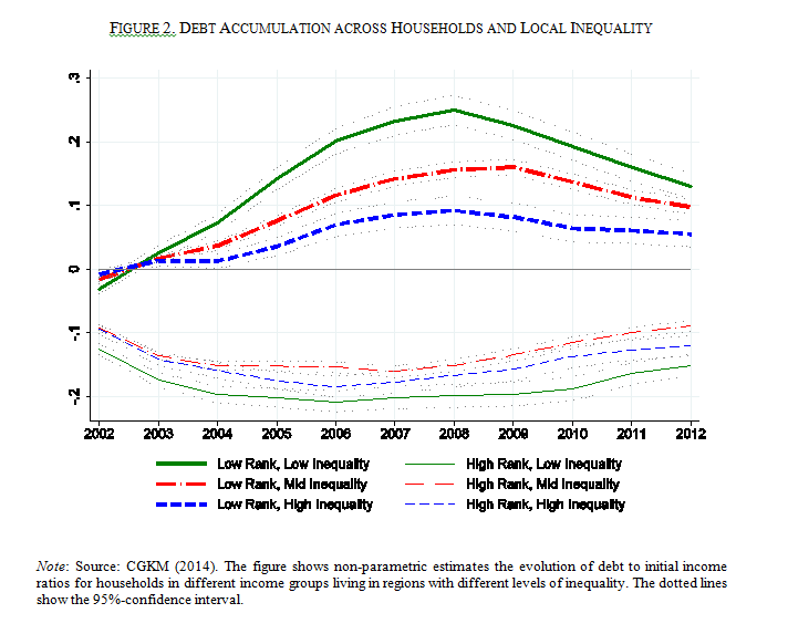
income inequality in their region. Our main finding is that low-income households
in high-inequality areas increased their leverage by less than similar
households in low-inequality areas. Our non-parametric results in Figure 2
suggest that a household in the bottom third of the income distribution within
their area and inequality distribution across areas increased their leverage by
around 15 percentage points more than a similar household in the top third of
the inequality distribution in the years immediately prior to the financial
crisis. This is the exact opposite effect one would expect if “keeping up with
the Joneses” was the primary cause of borrowing by low-income households.
Because our data (see Additional Details below) allow us to
break debt into pieces, we can examine which types of debt are driving these
differences. While we find similar patterns for mortgage debt, auto debt, and
credit card limits as those documented for total debt accumulation, we find no
systematic differences across households and inequality regions in terms of
their credit card balances. Since credit card limits primarily reflect credit
supply conditions whereas credit card balances reflect households’ demand for
credit, we interpret the difference in results across credit card limits and
balances as pointing toward credit supply factors as the root cause of the link
between inequality and borrowing.
The intuition is simple. First, lenders confront asymmetric
information as they try to infer which borrowers are less likely to default.
Second, high-income borrowers are less likely to default so lenders use income
as a way to infer borrower type. In a perfectly equal income distribution all
borrowers are equally likely to be a high or low default risk. But as
inequality increases and the income difference between low- and high-income
borrowers becomes larger, high-risk and low-risk borrowers are easier to tell
apart when they reveal their incomes to banks. Lenders will then be able to
offer cheaper and more readily accessible credit to high-income/low-risk
borrowers as well as more likely to deny loans to low-income/high-risk
borrowers. To test these predictions we use data from the Home Mortgage
Disclosure Act (HMDA) which requires mortgage lenders to report details on
applications including whether a loan was denied, the size of the loan, income
of the applicant, and other characteristics. We find that low-income applicants
are more likely to be denied mortgages and to be charged a high interest rate
in high-inequality areas relative to similar applicants in low-inequality
areas. Thus, this evidence also supports a credit supply interpretation of the
link between local income inequality and differential borrowing patterns across
income groups that is at odds with the “keeping up with the Joneses”
interpretation.
Part of the reason I was invited to write here was to
discuss the differences between our results and those in a recent paper by
Bertrand and Morse, because their empirical findings do provide evidence
of “keeping up with the Joneses” forces. There are at least two important
differences. First, their outcome is consumption while ours is debt. It is
possible that low-income households funded their consumption with changes in
labor supply, savings, or even some debt. But our results tell us that any use
of debt in this way cannot be the primary story of inequality and debt
accumulation during this period. This is important to note because debt
accumulation was central to the creation of many of the financial assets behind
the financial crisis. Second, Bertrand and Morse use changes in consumption
among the wealthy as their explanatory variable while we use inequality. It is
possible that in some areas the consumption differences between households are
not as large as in other areas even though both have the same measured
inequality. This can occur if there is variation in precautionary savings, the
“visibility” of consumption bundles, or the proximity of high- and low-income
households. As the relationship between high-income household consumption and
measured inequality becomes more complex our results become less directly
comparable.
Thanks very much to Carola for having us!
Additional Details
The data we use for our primary results are from the New York Federal Reserve Bank Consumer Credit Panel/Equifax (referred to as the CCP), which provides comprehensive debt measures for millions of U.S. households since 1999. Because these data do not include income we impute incomes using the relationship between common observables in the Survey of Consumer Finances. Using these imputed incomes we construct measures of local inequality, household positions in the income distribution, and household debt-to-income ratios. We are able to check our measures of inequality and rank against various external measures and find they are very highly correlated.
Our results are robust to the level at which we measure inequality (zip, county, state), the measure of inequality we use (ratio of log incomes at the 90th and 10th percentile from the CCP, Gini coefficients from the IRS and Census data), an extensive set of household and area controls, and numerous splits of our sample. In particular our results hold within subsamples defined according to house price appreciation, average credit scores, income levels, initial debt ratios, and geographic regions.
This comment has been removed by a blog administrator.
ReplyDeleteThis comment has been removed by a blog administrator.
ReplyDeleteMany thanks for the amazing essay I really gained a lot of info. That I was searching for
ReplyDelete
ReplyDeleteMany thanks for the amazing essay I really gained a lot of info. That I was searching for
ReplyDeleteMany thanks for the amazing essay I really gained a lot of info. That I was searching for